Ordinary Differential Equations

Differential Equations: ODEs and PDEs

Differential equations are a fundamental concept in mathematics and play a crucial role in various fields of science and engineering, including physics, biology, economics, and computer science. Differentail equations provide a powerful framework for modeling and analyzing dynamic systems.

At its core, a differential equation is an equation that relates an unknown function \(y(t)\) to its derivatives \(\frac{dy}{dt}\). These equations express relationships between the rates of change of a quantity and the quantity itself. Differential equations can describe a wide range of phenomena, from the motion of celestial bodies to the spread of diseases in populations.

There are two main types of differential equations: ordinary differential equations (ODEs) and partial differential equations (PDEs).

ODEs involve functions of a single variable, typically representing time \(t\). Mathematically, an ordinary differential equation (ODE) can be represented as:

If we want to follow formalities, an ordinary differential equaltion is an equation involving a function of one variable and at least one of its derivatives, i.e. an ODE for the function \(y(x)\) may be written in the form \(G\left(x, y(t), \frac{dy}{dt}, ..., \frac{d^ny}{dt^n} \right) =0\) for some function \(G\) and some positive integer \(n\). The order of an ODE is the order of the highest order derivative that it contains.

\[ \frac{dy}{dt} = f(t,y), \]

where \(y\) is the unknown function of \(t\), and \(f(t,y)\) is a givem function definiging the relashionship between \(y\) and its derivatives.

PDEs involve functions of multiple variables \(\theta=(\theta_1, ..., \theta_k)\) and their partial derivatives \(\frac{\partial f}{d \theta_i}\). Both types of equations arise frequently in computational problems, and various numerical methods have been developed to solve them efficiently.

Analytical methods for solving ODEs

There are several methods to solve ordinary differential equations (ODEs) analytically, depending on the type of equation and its properties. Here’s a list of some common methods:

• Separation of Variables: suitable for first-order ODEs where the variables can be separated into different sides of the equation and integrated individually.

• Exact Equations: a method to solve first-order ODEs which are exact differentials, meaning they can be expressed as the total differential of some function.

• Integrating Factors: a technique to solve first-order linear ODEs that are not exact by finding a suitable integrating factor that makes the equation exact.

• Substitution Methods: involves substituting a new variable or function to transform the given ODE into a simpler form that can be solved more easily.

• Homogeneous Equations: used to solve first-order ODEs where the right-hand side can be expressed as a function of the ratio of the dependent and independent variables.

• Linear ODEs with Constant Coefficients: solvable using methods like the method of undetermined coefficients, variation of parameters, or the annihilator method.

• Power Series Solutions: useful for solving ODEs where the solution can be expressed as a power series.

• Fourier Series and Transforms: Can be used for solving ODEs defined on intervals or with periodic boundary conditions.

• Reduction of Order: a technique used to reduce higher-order ODEs to first-order ODEs by introducing new variables.

and more.

Let us consider some examples.

Separation of Variables

This technique is often used to solve first-order ordinary differential equations (ODEs). The idea is to rearrange the equation so that variables can be separated on either side of the equation and then integrate both sides. For example, consider the separable ODE:

\[ \frac{dy}{dt} = f(t) \cdot g(y) \]

By separating variables, we can write:

\[ \frac{dy}{g(y)} = f(t) \cdot dt \]

Then, integrating both sides yields the solution.

Separation of Variables: example

Consider the following first-order ordinary differential equation (ODE):

\[ \frac{dy}{dt} = t \cdot y \]

We can solve this equation using separation of variables. First, let’s separate the variables by moving all terms involving \(y\) to one side and all terms involving \(t\) to the other side:

\[ \frac{dy}{y} = t \cdot dt \]

Next, we integrate both sides of the equation:

\[ \int \frac{1}{y} \, dy = \int t \, dt \]

Integrating the left side with respect to \(y\) yields \(\ln|y|\), and integrating the right side with respect to \(t\) yields \(\frac{1}{2} t^2 + C\) (where \(C\) is the constant of integration). So we have:

\[ \ln|y| = \frac{1}{2} t^2 + C \]

To find the solution for \(y\), we exponentiate both sides:

\[ |y| = e^{\frac{1}{2} t^2 + C} = Ce^{\frac{1}{2} t^2} \]

where \(C\) is the constant of integration. Since \(|y|\) can be positive or negative, we keep the absolute value on the left side. Thus, the general solution to the differential equation is:

\[ y(t) = Ce^{\frac{1}{2} t^2} \]

where \(C\) is an arbitrary constant.

Now consider the same ODE, but this time with an initial condition:

\[ \frac{dy}{dt} = t \cdot y, \quad y(0) = y_0. \]

We can now determine the constance \(C\) by applying the initial condition ( y(0) = y_0 ):

\[ |y_0| = Ce^{\frac{1}{2} \cdot 0^2} = C \]

So, \(C = |y_0|\). Thus, the solution to the differential equation with the given initial condition is:

\[ y(t) = |y_0| e^{\frac{1}{2} t^2} \]

where \(y_0\) is the initial value of \(y\) at \(t = 0\).

Exact Equations

The method of exact equations is used to solve first-order ordinary differential equations (ODEs) that can be expressed as the total differential of some function. These equations have the form:

\[ M(x, y) \, dx + N(x, y) \, dy = 0 \]

Where \(M\) and \(N\) are functions of \(x\) and \(y\).

The differential equation is called exact if there exists a function \(F(x, y)\) such that:

\[ \frac{\partial F}{\partial x} = M \quad \text{and} \quad \frac{\partial F}{\partial y} = N \]

If this condition holds, then the equation can be written as:

\[ dF = \frac{\partial F}{\partial x} \, dx + \frac{\partial F}{\partial y} \, dy = 0 \]

This means that the left-hand side of the original equation is an exact differential, and hence \(F(x, y) = C\) (where \(C\) is a constant) represents the general solution to the differential equation.

The step-by-step procedure to solve an exact differential equation is as follows:

• Check for Exactness: Verify if the equation is exact by checking if \(\frac{\partial M}{\partial y} = \frac{\partial N}{\partial x}\). If this condition holds, proceed to the next step. If not, the equation is not exact and other methods must be considered.

• Find the Integrating Factor: If the equation is not exact, it may be possible to find a suitable integrating factor \(\mu(x, y)\) such that when the equation is multiplied by \(\mu\), it becomes exact. The integrating factor is typically found as \(\mu(x, y) = e^{\int P(x) \, dx}\) or \(\mu(x, y) = e^{\int Q(y) \, dy}\), where \(P(x)\) and \(Q(y)\) are functions that depend only on \(x\) or \(y\), respectively.

• Solve for \(F(x, y)\): If the equation is exact or has been made exact using an integrating factor, find \(F(x, y)\) by integrating \(M\) with respect to \(x\) or \(N\) with respect to \(y\), depending on which derivative yields \(F\).

• General Solution: Once \(F(x, y)\) is found, the general solution is given by \(F(x, y) = C\), where \(C\) is a constant.

• Boundary Conditions (if any): If initial conditions or boundary conditions are given, use them to determine the value of the constant \(C\) and obtain the particular solution.

The method of exact equations is particularly useful when dealing with certain types of first-order ODEs where other methods may be less applicable.

Exact Equations: example

Consider the first-order ordinary differential equation (ODE):

\[ 2xy \, dx + (x^2 + 1) \, dy = 0 \]

We’ll solve this equation using the method of exact equations.

• Check for Exactness: Compute the partial derivatives of \(M(x, y) = 2xy\) with respect to \(y\) and \(N(x, y) = x^2 + 1\) with respect to \(x\):

  \(\frac{\partial M}{\partial y} = 2x \quad \text{and} \quad \frac{\partial N}{\partial x} = 2x\)

  Since \(\frac{\partial M}{\partial y} = \frac{\partial N}{\partial x}\), the equation is exact.

• Find \(F(x, y)\): Integrate \(M\) with respect to \(x\) to find \(F(x, y)\):

  \(F(x, y) = \int 2xy \, dx = x^2y + g(y)\)

  Differentiate \(F(x, y)\) with respect to \(y\) and set it equal to \(N(x, y)\) to find \(g(y)\):

  \(\frac{\partial F}{\partial y} = x^2 + g'(y) = x^2 + 1\)

  Solving for \(g'(y)\), we get:

  \(g'(y) = 1 \implies g(y) = y + C\)

  Therefore, \(F(x, y) = x^2y + y + C\).

• General Solution

  The general solution is given by \(F(x, y) = x^2y + y + C = 0\), where \(C\) is a constant.

  This is the general solution to the given ODE using the method of exact equations. If initial conditions or boundary conditions were provided, they could be used to determine the value of the constant \(C\) and obtain the particular solution.

Integrating Factors

The integrating factor method is a technique used to solve first-order linear ordinary differential equations (ODEs) that are not exact by finding a suitable integrating factor that makes the equation exact. This method is particularly useful when the equation is not in a form where it can be solved directly using the method of exact equations. The method involves multiplying the original differential equation by a specific function (the integrating factor) to make it exact and then applying the method of exact equations to solve it.

Consider a first-order linear ordinary differential equation (ODE) of the form:

\[ \frac{dy}{dx} + P(x)y = Q(x) \]

The integrating factor, denoted by \(\mu(x)\), is a function of \(x\) that is chosen such that when the original equation is multiplied by it, the resulting equation becomes exact. The integrating factor \(\mu(x)\) is given by:

\[ \mu(x) = e^{\int P(x) \, dx} \]

Once the integrating factor is determined, the original equation is multiplied by it:

\[ \mu(x) \left( \frac{dy}{dx} + P(x)y \right) = \mu(x)Q(x) \]

\[ \frac{d}{dx} \left( \mu(x)y \right) = \mu(x)Q(x) \]

The left-hand side is now a total differential, which makes the equation exact. We can now proceed to solve the equation using the method of exact equations:

• Find \(F(x, y)\): Integrate \(\mu(x)Q(x)\) with respect to \(x\) to find the function \(F(x, y)\) such that \(\frac{\partial F}{\partial x} = \mu(x)Q(x)\).

• General Solution: integrate both sides with respect to \(x\).

• Boundary Conditions (if any): If initial conditions or boundary conditions are given, use them to determine the value of the constant \(C\) and obtain the particular solution. \end{enumerate}

The integrating factor method is particularly useful for solving linear ODEs with variable coefficients, where the method of exact equations may not be directly applicable. It transforms the original equation into an exact equation, allowing for the application of standard techniques for solving such equations.

Integrating Factors: example

Consider the first-order linear ordinary differential equation (ODE) given by:

\[ \frac{dy}{dt} + 2ty = t^2 \]

To solve this equation using the integrating factor method, we first identify the coefficient of \(y\) as \(2t\), which is a function of \(t\). The integrating factor \(\mu(t)\) is then defined as \(e^{\int 2t \, dt}\).

\[ \mu(t) = e^{\int 2t \, dt} = e^{t^2} \]

Next, we multiply both sides of the ODE by the integrating factor \(I(t)\):

\[ e^{t^2} \frac{dy}{dt} + 2te^{t^2}y = t^2e^{t^2} \]

The left-hand side can now be recognized as the result of applying the product rule to \(e^{t^2}y\), giving:

\[ \frac{d}{dt}(e^{t^2}y) = t^2e^{t^2} \]

Now, we integrate both sides with respect to \(t\):

\[ \int \frac{d}{dt}(e^{t^2}y) \, dt = \int t^2e^{t^2} \, dt \]

\[ e^{t^2}y = \int t^2e^{t^2} \, dt + C \]

To find the expression for \(y\), we integrate the right-hand side:

\[ y = e^{-t^2} \int t^2e^{t^2} \, dt + Ce^{-t^2} \]

To evaluate the integral \(\int t^2e^{t^2} \, dt\), we can use a simple substitution. Let \(u = t^2\), then \(du = 2t \, dt\). The integral becomes:

\[ \int t^2e^{t^2} \, dt = \frac{1}{2} \int e^u \, du = \frac{1}{2} e^{t^2} + K \]

A general solution of an ODE represents all possible solutions to the equation, typically expressed with arbitrary constants that can take on any value within a specified range. A particular solution of an ODE is a specific solution that satisfies both the differential equation and any given initial or boundary conditions. Unlike a general solution, which encompasses all possible solutions with arbitrary constants, a particular solution is unique for a given set of conditions.

Substituting this back into our equation for \(y\), we get:

\[ y = \frac{1}{2} t^2 + K \]

where \(K\) is a constant. Thus, we have found the general solution to the differential equation.

This method has transformed the original first-order linear ODE into an integrable form. By completing the integration, we can obtain the general solution to the differential equation.

Numerical methods for solving ODEs

Solving and ODE by hand is not always possible.

Numerical methods provide powerful tools for solving ODEs when analytical solutions are difficult or impossible to obtain. These methods involve discretizing the differential equation and approximating the solution at discrete points in the domain.

One of the simplest numerical methods is Euler’s method, which iteratively computes the solution at successive points based on the local slope of the function.

More accurate methods include the Runge-Kutta methods, such as the classical fourth-order Runge-Kutta method (RK4), which improve upon Euler’s method by considering multiple slope estimates within each step. Additionally, there are adaptive methods like the Dormand-Prince method that automatically adjust the step size to control accuracy while minimizing computational cost.

Let’s consider the following first-order ODE:

Make sure that you can solve this ODE analytically. What is its solution?

\[ \frac{dy}{dx} = -2x + 1. \]

We will solve this equation using the odeint function from the scipy.integrate module.

Note that we import bothe odeint as odeint_scipy from scipy.integrate, as well as scipy from jax.experimental.ode.

import numpy as np
from scipy.integrate import odeint as odeint_scipy

import numpyro
import numpyro.distributions as dist
from numpyro.infer import MCMC, NUTS

import jax
import jax.numpy as jnp
from jax.experimental.ode import odeint

import matplotlib.pyplot as plt
import seaborn as sns

/opt/hostedtoolcache/Python/3.11.9/x64/lib/python3.11/site-packages/tqdm/auto.py:21: TqdmWarning: IProgress not found. Please update jupyter and ipywidgets. See https://ipywidgets.readthedocs.io/en/stable/user_install.html
  from .autonotebook import tqdm as notebook_tqdm

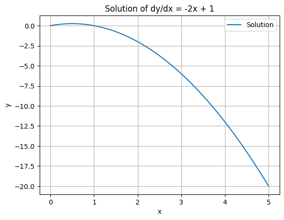
# Define the function that represents the differential equation dy/dx = -2x + 1
def model(y, x):
    return -2*x + 1

# Initial condition
y0 = 0

# Array of x values
x = np.linspace(0, 5, 100)

# Solve the ODE using odeint
y = odeint_scipy(model, y0, x)

# Plot the solution
plt.plot(x, y, label='Solution')
plt.xlabel('x')
plt.ylabel('y')
plt.title('Solution of dy/dx = -2x + 1')
plt.grid(True)
plt.legend()
plt.show()

In this example:

• We define the function model(y, x) that represents the differential equation.

• We specify the initial condition y0 at x=0.

• We create an array x of values where we want to compute the solution.

• We use the odeint function to solve the ODE, passing the model function, initial condition, and array of x values.

• Finally, we plot the solution.

ODEs in Numpyro.

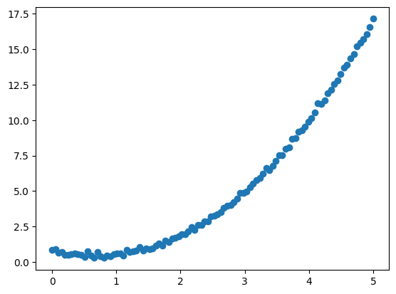
# Define the ordinary differential equation (ODE)
def ode(y, x):
    return x ** 2 - y

# Generate synthetic data
x_obs = jnp.linspace(0, 5, 100)
y0_true = 0.8
true_y = odeint(ode, y0_true, x_obs)  # True solution with initial condition y(0) = 0.5
observed_data = true_y + np.random.normal(0, 0.1, size=true_y.shape)  # Add noise

plt.scatter(x_obs, observed_data, label='observed data')

<matplotlib.collections.PathCollection at 0x7fd1d3e5b650>

# Define the probabilistic model representing the ODE
def model(y_obs=None):
    # Prior distribution for the initial value y(0)
    y0 = numpyro.sample('y0', dist.Normal(0., 1.))
    
    # Solve the ODE using numerical integration
    y = odeint(ode, y0, x_obs)
    sigma = numpyro.sample('sigma', dist.Exponential(1.))
    
    # Observation likelihood
    if y_obs is not None:
        numpyro.sample('obs', dist.Normal(y, sigma), obs=y_obs)

# Perform inference
nuts_kernel = NUTS(model)
mcmc = MCMC(nuts_kernel, num_samples=1000, num_warmup=500, progress_bar=False)
mcmc.run(rng_key=jax.random.PRNGKey(0), y_obs=jnp.array(observed_data))

# Extract posterior samples
posterior_samples = mcmc.get_samples()

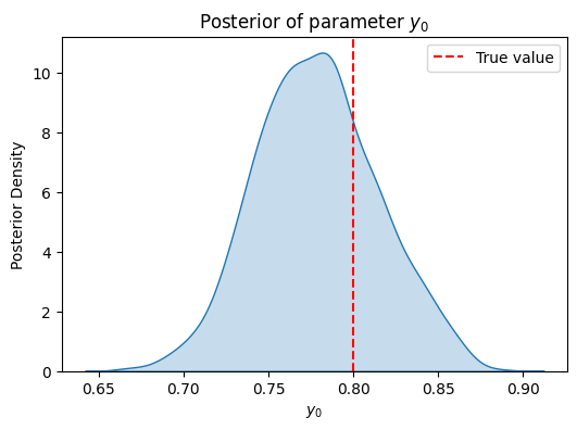
plt.figure(figsize=(6, 4))
sns.kdeplot(posterior_samples['y0'], fill=True)
plt.axvline(x=y0_true, color='r', linestyle='--', label='True value')
plt.xlabel('$y_0$')
plt.ylabel('Posterior Density')
plt.title('Posterior of parameter $y_0$')
plt.legend()

# Show the plot
plt.show()