Introduction to NumPyro

NumPyro [Bingham et al., 2019, Phan et al., 2019] is a probabilistic programming library that combines the flexibility of numpy with the probabilistic modelling capabilities of pyro, making it an excellent choice for researchers and data scientists. In this introductory tutorial, we’ll explore the basics of numpyro and how to get started with probabilistic programming in a hands-on manner.

Components of a Numpyro program

In a NumPyro program, you define a probabilistic model that consists of various elements. Let’s break down the key elements of a typical program using NumPyro:

1. Importing Libraries:

At the beginning of your NumPyro program, you import the necessary libraries, including NumPyro and other required dependencies like JAX. For example:

import numpy as np

import numpyro
import numpyro.distributions as dist
from numpyro.infer import MCMC, NUTS, Predictive
from numpyro.diagnostics import hpdi

import jax
import jax.numpy as jnp

# check number of devices available
num_device = jax.local_device_count()
print("Number of available devices: ", num_device)
numpyro.set_host_device_count(1)

import arviz as az

import matplotlib.pyplot as plt

/opt/hostedtoolcache/Python/3.11.10/x64/lib/python3.11/site-packages/tqdm/auto.py:21: TqdmWarning: IProgress not found. Please update jupyter and ipywidgets. See https://ipywidgets.readthedocs.io/en/stable/user_install.html
  from .autonotebook import tqdm as notebook_tqdm

Number of available devices:  1

2. Defining the Model Function:

In NumPyro, you define your probabilistic model as a Python function. This function encapsulates the entire model, including both the prior distributions and the likelihood. Typically, the model function takes one or more arguments, such as data or model parameters, and returns a set of latent variables and observations.

def model():
    pass

3. Prior Distributions:

Inside the model function, you define prior distributions for the model parameters. These prior distributions represent your beliefs about the parameters before observing any data. You use the numpyro.sample function to specify these priors. For example, in mean = numpyro.sample("mean", dist.Normal(0, 1)) and scale = numpyro.sample("scale", dist.Exponential(1)) within a function define mean and scale as random variables sampled from specific prior distributions.

4. Likelihood:

After specifying the prior distributions, you define the likelihood of your observed data by adding obs=data to the sampling statement of a variable. The likelihood represents the probability distribution of your observed data given the model parameters. It describes how likely it is to observe the data under different parameter values. In the example below, the numpyro.sample function is used to define the likelihood of the data points given the mean and scale parameters.

def model(data):
    
    # define prior distributions for model parameters
    mean = numpyro.sample("mean", dist.Normal(0, 1))
    scale = numpyro.sample("scale", dist.Exponential(1))

    # define likelihood
    numpyro.sample("obs", dist.Normal(mean, scale), obs=data)

5. Inference Algorithm:

After defining your model, you need to choose an inference algorithm to estimate the posterior distribution of model parameters. NumPyro supports various inference algorithms, including NUTS (No-U-Turn Sampler) and SVI (Stochastic Variational Inference). You initialize and configure the chosen inference algorithm according to your requirements.

nuts_kernel = NUTS(model)

6. Performing Inference:

You use the configured inference algorithm to perform Bayesian inference. In the example, Markov Chain Monte Carlo inference is performed using the MCMC class. The run method of the MCMC object is called to run the inference process.

I have set here progress_bar=False to reduce amount of output in the resulting html of the lecture file. In practice, you often want to set the value to True to know how long the model will still take to complete.

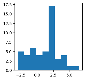
# generate data
mean_true = 1.0  
scale_true = 2.0  
n = 50
normal_dist = dist.Normal(mean_true, scale_true)
data = normal_dist.sample(jax.random.PRNGKey(8), (n,))

# plot data
plt.figure(figsize=(3, 3))
plt.hist(data)
plt.show()

# data
#data = jnp.array([2.3, 3.9, 1.7, -0.8, 2.5])

# use `chain_method='parallel'` to run multiple chains in parallel
if num_device > 1:
    mcmc = MCMC(nuts_kernel, num_samples=1000, num_warmup=1000, num_chains=num_device, chain_method='parallel', progress_bar=False)
else:        
    mcmc = MCMC(nuts_kernel, num_samples=1000, num_warmup=1000, num_chains=2, chain_method='sequential', progress_bar=False)
    
mcmc.run(jax.random.PRNGKey(0), data)

Note that the in the call above, we provided the number of chains num_chains=2, number of samples num_samples=1000 and number of warm-up samples num_warmup=1000.

7. Posterior Analysis:

After running the inference, you can retrieve posterior samples of the model parameters. These samples represent the estimated posterior distribution of the parameters given the observed data. You can then analyze these samples to make inferences about your model.

# get the posterior samples
posterior_samples = mcmc.get_samples()

# print summary statistics of posterior
mcmc.print_summary()

                mean       std    median      5.0%     95.0%     n_eff     r_hat
      mean      1.25      0.27      1.25      0.81      1.66   1068.07      1.00
     scale      1.94      0.19      1.92      1.63      2.25   1219.43      1.00

Number of divergences: 0

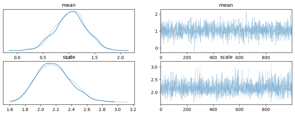
8. Visualizing inference results

Finally, you can perform various tasks such as visualizing the posterior distributions, computing summary statistics, and making predictions or inferences based on the posterior samples.

# visualise posterior distributions and trace plots
az.plot_trace(mcmc)

array([[<Axes: title={'center': 'mean'}>,
        <Axes: title={'center': 'mean'}>],
       [<Axes: title={'center': 'scale'}>,
        <Axes: title={'center': 'scale'}>]], dtype=object)

9. plate for repetition

We often work with multiple data points that share the same statistical structure. In such cases you might want to, or need to, use plates. The numpyro.plate context manager allows you to create a plate, which represents a repeated structure for data. It’s used to efficiently handle repeated observations. In the example, numpyro.plate is used to specify that the likelihood applies to multiple data points.

def model(data):
    
    # define prior distributions for model parameters
    mean = numpyro.sample("mean", dist.Normal(0, 1))
    scale = numpyro.sample("scale", dist.Exponential(1))

    # define likelihood with a data plate
    with numpyro.plate("data_plate", len(data)):
        obs = numpyro.sample("obs", dist.Normal(mean, scale), obs=data)

nuts_kernel = NUTS(model)

mcmc = MCMC(nuts_kernel, num_samples= 100, num_warmup= 100, num_chains=2, chain_method='sequential', progress_bar=False)
mcmc.run(jax.random.PRNGKey(0), data)

# get the posterior samples
posterior_samples = mcmc.get_samples()

# print summary statistics of posterior
mcmc.print_summary()

                mean       std    median      5.0%     95.0%     n_eff     r_hat
      mean      1.24      0.25      1.22      0.86      1.67    167.29      1.01
     scale      1.94      0.18      1.94      1.61      2.20    187.48      1.00

Number of divergences: 0

10. Get the last state last_state, and continue

mcmc.post_warmup_state = mcmc.last_state 
mcmc.run(mcmc.post_warmup_state.rng_key, data)

# get the posterior samples
new_posterior_samples = mcmc.get_samples()

# print summary statistics of posterior
mcmc.print_summary()

                mean       std    median      5.0%     95.0%     n_eff     r_hat
      mean      1.24      0.25      1.23      0.87      1.61    116.97      1.00
     scale      1.96      0.22      1.96      1.62      2.27    147.24      1.00

Number of divergences: 0

11. Custom likelihood with numpyro.factor

Not all distributions we might need would be implemented in Numpyro. In such cases, we can implement custom ones using numpyro.factor. This primitive allows to add arbitrary log-probability terms to the model.

Assume we would like to implement a distribution which is a mixture of Normal and Laplace distributions. We compute the log-likelihood manually and use numpyro.factor to incorporate it into the model.

def model(data = None):
    mean = numpyro.sample("mean", dist.Normal(0, 5))
    scale = numpyro.sample("scale", dist.LogNormal(0, 1))
    
    # compute the log-probabilities for each data point
    normal_log_probs = dist.Normal(mean, scale).log_prob(data)
    laplace_log_probs = dist.Laplace(mean, scale).log_prob(data)
    
    # mixture log-probability: log(0.7 * p1 + 0.3 * p2)
    log_mixture_probs = jnp.log(0.7 * jnp.exp(normal_log_probs) + 0.3 * jnp.exp(laplace_log_probs))
    
    # sum the log-probabilities across all data points
    total_log_prob = jnp.sum(log_mixture_probs)
    
    # add to the model using `numpyro.factor`
    numpyro.factor("custom_log_likelihood", total_log_prob)


nuts_kernel = NUTS(model)
mcmc = MCMC(nuts_kernel, num_warmup=500, num_samples=1000, progress_bar=False)
mcmc.run(jax.random.PRNGKey(0), data = data)

mcmc.print_summary()

                mean       std    median      5.0%     95.0%     n_eff     r_hat
      mean      1.39      0.28      1.38      0.94      1.83    840.73      1.00
     scale      1.78      0.21      1.77      1.46      2.14    463.73      1.00

Number of divergences: 0

Summary

The typical elements that we will need to write a model in Numpyro are as follows:

• sample parameters with numpyro.sample,

• sample parameters from any of the built-in distributions using, e.g. dist.Beta(alpha, beta),

• specify likelihood by adding obs=... to the sampling statement: numpyro.sample('obs', dist.Binomial(n, p), obs=h),

• specify a sampling algorithm. NUTS is a good default option: kernel = NUTS(model) ,

• specify number of warm-up steps, number of iterations, number of chains, e.g. MCMC(kernel, num_warmup=1000, num_samples=2000, num_chains=4),

• use Predictive class we can generate predictions,

• use numpyro.factor to implement custom distributions.

Task 16

• You might have correctly noticed that we have not looked at the Predictive capability. Study the documentation of Numpyro (in particular, numpyro.infer) and demonstrate the Predictive command on the example shown above.

• Study the documentation of Numpyro (in particular, numpyro.diagnostics) to understand what the hpdi command does. Apply it to the example shown above.

• Look up documentation of mcmcm.last_state and explain what it is doing.

Outro

NumPyro is a versatile library for probabilistic programming that combines the power of NumPy and Pyro. In this introductory tutorial, we’ve covered the basics of defining a probabilistic model, performing MCMC inference, and visualizing the results. As you delve deeper into probabilistic programming with NumPyro, you’ll be able to build more complex and customized models for your specific applications. Happy modelling!