Hierarchical modelling

Why are linear models not enough?

The linear models which we considered earlier have a set of assumptions behind them which are not always realistic. Such assumptions may enable analytical derivations in some cases, but these simplifications might be too limiting when we need to model real-life data.

Epidemiological data is often complex, and we need to have appropriate tools to model complexity.

Group Task

Discuss with your neighbours how exactly the assumption of indendepdent errors \(\epsilon_i\) in linear regression \(y_i = X_i \beta + \epsilon_i, \quad \epsilon_i \sim \mathcal{N}(0, \sigma^2)\) helps in the classical setting. What does it enable us to compute analytically?

One of the simplifying assumptions is homoskedasticity, i.e. the assumption of equal or similar variances in different groups.

Sometimes it is indeed appropriate, but very often it is not.

Here is a wider list of assumptions made by linear models:

• homoskedasticity: equal or similar variances in different groups,

• no error in predictors \(X\),

• no missing data,

• normally distributed errors,

• observations \(y_i\) are independent.

What we would often like to do, however, is

• to model variance,

• to capture errors in variables,

• to allow for missing data,

• use generalised linear models (GLMs),

• use spatial and/or temporal error structure imposing correlation structure.

Hierarchies in data and parameters

Hierarchical structures are commonly found in both natural data and statistical models. These hierarchies can represent various levels of organization or grouping within the data, and incorporating them into Bayesian inference can provide more accurate and insightful results. Such approach to modelling allows to account for different sources of variation in the data.

The hierarchical structure often arises in problems such as multiparameter models, where parameters can be regarded or connected in some way, or models of complex phenomena with different levels of hierarchy in the data.

Hierarchical models are also often called multilevel models.

Generally, a hierarchical structure can be written if the joint distribution of the parameters can be decomposed to a series of conditional distributions. The term hierarchical models refers to a general set of modelling principles rather than to a specific family of models.

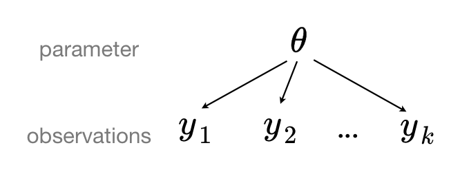
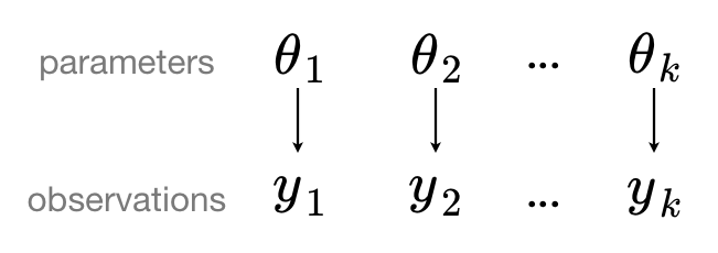
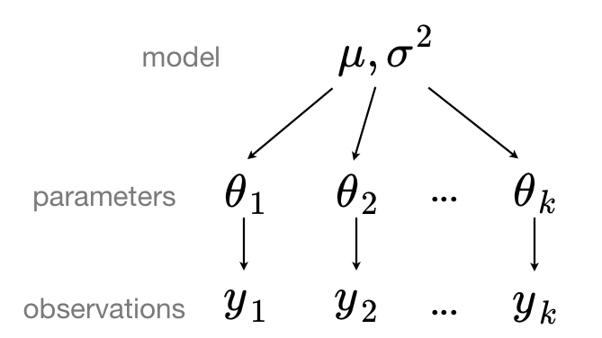
Priors of model parameters are the first level of hierarchy. Priors of model parameters can depend on other parameters, and new priors (hyperpriors) are defined over these prior parameters. In this case, the hyperpriors would be the second level of hierarchy. Following this scheme, the structure can be extended to more levels of hierarchy. In principle, there is not a limited level of hierarchy.

Let us illustrate in an equation the posterior distribution of a model parameter with conditional structure and two levels of hierarchy. The prior distribution of model parameter \(\theta\), \(p(\theta|a)\), depends on the parameter \(a\); the hyperprior \(p(a|b)\) depends on a fixed value \(b\) (hyper-parameter).

\[ p(\theta|y) \propto p(y|\theta)p(\theta|a)p(a|b). \]

The sampling order in this example follows the computational graph:

\[\begin{split} \begin{array}{c} b\\ \downarrow\\ a\\ \downarrow\\ \theta\\ \downarrow\\ y \end{array} \end{split}\]

Here is a more specific example of hierarchical structure:

\[\begin{split} \begin{align*} \text{likelihood: } \quad &p(y_i | \mu_i, \sigma) &&= \mathcal{N}(y_i | \mu_i, \sigma), \\ \text{prior: } \quad &p(\mu_i) &&= \mathcal{N}(\mu_i | 0, \sigma_\mu)\\ \text{prior: } \quad &p(\sigma| a) &&= \mathcal{HalfCauchy}(\sigma|a)\\ \text{hyperprior: } &p(\sigma_\mu) &&= \mathcal{HalfCauchy}(\sigma_\mu|b) \end{align*} \end{split}\]

Due to their flexibility, hierarchical models allow us to model variability in the parameters of the model, partition variability more explicitly into multiple terms, ”borrow strength” across groups.

Levels of pooling

Hierarchical models exist on the continuum of two extreme cases: complete pooling and no pooling. In-between the two extremes is partial pooling.

Let’s explore each of these approaches and provide Numpyro code examples.

Complete Pooling

In the “complete pooling” approach, all data points are treated as if they belong to a single group or population, and the model estimates a single set of parameters for the entire dataset.

A pooled model implies that the data are sampled from the same model. This ignores all variation among the units being sampled. All observations share common parameter \(\theta\):

Image credit: Chris Fonnesbeck

Making predictions from a complete pooling model is straightforward.

import numpyro
import numpyro.distributions as dist
from numpyro.infer import MCMC, NUTS

import jax
from jax import random
import jax.numpy as jnp

rng_key = random.PRNGKey(678)

import pandas as pd

import matplotlib.pyplot as plt

/opt/hostedtoolcache/Python/3.11.9/x64/lib/python3.11/site-packages/tqdm/auto.py:21: TqdmWarning: IProgress not found. Please update jupyter and ipywidgets. See https://ipywidgets.readthedocs.io/en/stable/user_install.html
  from .autonotebook import tqdm as notebook_tqdm

# artificial data for us to work with
data = jnp.array([10, 12, 9, 11, 8]) # remember to turn data into a jnp array

# Model
def complete_pooling_model(data):
    mu = numpyro.sample("mu", dist.Normal(0, 10))
    sigma = numpyro.sample("sigma", dist.Exponential(1))
    obs = numpyro.sample("obs", dist.Normal(mu, sigma), obs=data)

# Inference
nuts_kernel = NUTS(complete_pooling_model)
mcmc = MCMC(nuts_kernel, num_samples=1000, num_warmup=500, progress_bar=False)
mcmc.run(rng_key, data)

# Note how many mu-s and sigma-s are estimated
mcmc.print_summary()

                mean       std    median      5.0%     95.0%     n_eff     r_hat
        mu      9.92      0.77      9.94      8.64     11.13    460.42      1.00
     sigma      1.65      0.53      1.55      0.93      2.37    388.83      1.00

Number of divergences: 0

This approach assumes that there is no variation between data points, which can be overly restrictive when there is actual heterogeneity in the data.

No Pooling

In the “no pooling” approach, each data point is treated independently without any grouping or hierarchical structure. This approach assumes that there is no shared information between data points, which can be overly simplistic when there is underlying structure or dependencies in the data.

Image credit: Chris Fonnesbeck

Making predictions for new data from a no pooling model is impossible since it assumes no relashionship between the previously observed and new data.

# Model
def no_pooling_model(data):
    for i, obs in enumerate(data):
        mu_i = numpyro.sample(f"mu_{i}", dist.Normal(0, 10))
        sigma_i = numpyro.sample(f"sigma_{i}", dist.Exponential(1))
        numpyro.sample(f"obs_{i}", dist.Normal(mu_i, sigma_i), obs=data[i])

# Inference
nuts_kernel = NUTS(no_pooling_model)
mcmc = MCMC(nuts_kernel, num_samples=1000, num_warmup=500, progress_bar=False)
mcmc.run(rng_key, data)

# Note how many mu-s and sigma-s are estimated
mcmc.print_summary()

                mean       std    median      5.0%     95.0%     n_eff     r_hat
      mu_0      9.98      1.06     10.00      8.17     11.35    338.50      1.00
      mu_1     11.71      1.77     11.97      8.72     14.16    304.16      1.00
      mu_2      8.85      1.35      8.92      6.53     10.57    419.85      1.00
      mu_3     10.81      1.37     10.92      8.91     12.81    212.94      1.00
      mu_4      7.87      1.23      7.96      6.34      9.82    115.95      1.00
   sigma_0      0.94      0.82      0.67      0.08      2.02    259.38      1.00
   sigma_1      1.15      1.11      0.81      0.06      2.53    117.35      1.00
   sigma_2      1.10      0.99      0.85      0.07      2.29    242.58      1.01
   sigma_3      1.06      0.89      0.84      0.08      2.20    102.34      1.00
   sigma_4      1.01      0.91      0.80      0.05      2.12    147.39      1.00

Number of divergences: 120

Partial Pooling

In the “partial pooling” approach, the data is grouped into distinct categories or levels, and each group has its own set of parameters. However, these parameters are constrained by a shared distribution, allowing for both individual variation within groups and shared information across groups.

Image credit: Chris Fonnesbeck

Heart attack meta-analysis

Consider the data from a meta-analysis of heart attack data (it is from Draper, “Combining Information: Statistical Issues and Opportunities for Research”, 1992).

Each data point represents the outcome of a study on post-heart attack survivorship. Each study involved administering aspirin to some victims immediately after the heart attack, while others did not receive aspirin. The y values denote the differences in mean survivorship observed in each study. Moreover, each study provided a standard deviation, calculated based on the relative sizes of the two groups within the study.

# Data
y = jnp.array([2.77, 2.50, 1.84, 2.56, 2.31, -1.15])
sd = jnp.array([1.65, 1.31, 2.34, 1.67, 1.98, 0.90])

We can build a model

\[\begin{split} \begin{align*} y_i &\sim \mathcal{N}(\theta_i, s_i),\\ \theta_i &\sim \mathcal{N}(\mu, \tau), \end{align*} \end{split}\]

where \(y_i\) is the mean of each study, and \(s_i\) is the standard deviation for each study. Parameters \(\mu\) and \(\tau\) themselves can have priors

\[\begin{split} \begin{align*} \mu &\sim \mathcal{N}(\bar{y}, 10s_y),\\ \tau &\sim \mathcal{HalfCauchy}(5s_y). \end{align*} \end{split}\]

def model(y, sd):
    # hyperpriors
    mu = numpyro.sample('mu', dist.Normal(jnp.mean(y), 10*jnp.std(y)))
    tau = numpyro.sample('tau', dist.HalfCauchy(scale=5*jnp.std(y)))
    
    # prior
    theta = numpyro.sample('theta', dist.Normal(mu, tau), sample_shape=(len(y),))

    # Likelihood
    numpyro.sample('obs', dist.Normal(theta, sd), obs=y)

# Inference
nuts_kernel = NUTS(model)
mcmc = MCMC(nuts_kernel, num_samples=1000, num_warmup=500, progress_bar=False)
mcmc.run(jax.random.PRNGKey(0), y=y, sd=sd)

# Get posterior samples
posterior_samples = mcmc.get_samples()

# Print summary statistics
numpyro.diagnostics.print_summary(posterior_samples, prob=0.89, group_by_chain=False)

                mean       std    median      5.5%     94.5%     n_eff     r_hat
        mu      1.56      1.21      1.45     -0.17      3.27    530.82      1.00
       tau      1.93      1.17      1.70      0.43      3.10    326.78      1.00
  theta[0]      2.10      1.31      2.04      0.21      4.29    578.81      1.00
  theta[1]      2.11      1.12      2.04      0.38      3.92    668.76      1.00
  theta[2]      1.67      1.66      1.59     -0.97      4.28    733.75      1.00
  theta[3]      2.03      1.37      1.95     -0.01      4.26    551.78      1.00
  theta[4]      1.75      1.37      1.71     -0.18      4.29    678.10      1.00
  theta[5]     -0.45      0.91     -0.43     -1.87      0.92    466.13      1.00

On the level of data, hierarchies usually are expressed in terms of groups:

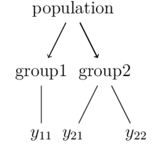
For example, \(y_{2j}\) here could represent repeated measurements within the same group.

Sleep study

Belenky, Gregory, Nancy J. Wesensten, David R. Thorne, Maria L. Thomas, Helen C. Sing, Daniel P. Redmond, Michael B. Russo, and Thomas J. Balkin. 2003. “Patterns of Performance Degradation and Restoration During Sleep Restriction and Subsequent Recovery: A Sleep Dose-Response Study.” Journal of Sleep Research 12: 1–12.

The aim of the sleep study was to assess the imapct of sleep deprivation on reaction time. The sleepstudy dataset consists of records of 18 subjects. All subjects got a regular night’s sleep on “day 0” of the study, and were then restricted to 3 hours of sleep per night for the next 9 days. Each day, researchers recorded the subjects’ reaction times (in ms) on a series of tests.

# To get the file using wget
# !wget -O sleepstudy.csv https://raw.githubusercontent.com/elizavetasemenova/prob-epi/main/data/sleepstudy.csv
# df = pd.read_csv('sleepstudy.csv')
# Drop the colum
# df = df.drop('Unnamed: 0', axis=1)
# df.head()


df = pd.read_csv('data/sleepstudy.csv')
# Drop the column
df = df.drop('Unnamed: 0', axis=1)
df.head()

	Reaction	Days	Subject
0	249.5600	0	308
1	258.7047	1	308
2	250.8006	2	308
3	321.4398	3	308
4	356.8519	4	308

Task 22

• Draw a diagram showing the hierarchy in the data. What are the “groups” here?

Complete pooling:

• Suppose that we took a complete pooling approach to modelling Reaction time (\(y\)) by Days of sleep deprivation (\(x\)). Draw a diagram of complete pooling.

• Ignore the subjects and fit the complete pooling model. Visualise the result.

No pooling:

• Construct and discuss separate scatterplots of Reaction by Days for each Subject.

• Fit the no pooling model to the data.

Partial pooling:

• Plot only data for subjects 308 and 335.

• For these two subjects, provide a loose sketch of three separate trend lines corresponding to a completely pooled, not pooled, and partially pooled model

• Fit a partially poolled model and visualise the results.

Task 23

Cushny, Arthur R., and A. Roy Peebles. “The action of optical isomers: II. Hyoscines.” The Journal of Physiology (1905)

The dataset sleep.csv contains results of a small clinical trial.

In this study, ten individuals were administered a sleep aid drug, followed by another sleep aid drug. The study tracked the additional hours of sleep each participant experienced under each drug regimen, relative to their baseline measurement.

The dataset is relatively small, with a low sample size and only one predictor variable (the treatment). Luckily, the design of the experiment has a hierarchical structure.

The data for this task can be loaded as follows:

df = pd.read_csv('data/sleep.csv')
df.head()

• Plot the data by showing treatment ID on the x-axis, and the number of extra hours of sleep on the y-axis. Add a separate line for each individual.

• Before fitting the model, what do you think the result will be: did drug 1 have an effect? did drug 2 have an effect?

• Construct a hierarchical model to analyse this data (you might want to consult this analysis for an example).

• What conclusions can you make from the analysis about drug 1 and drug 2?

Random effects

A common special case of hierarchical models are random effects.

Consider the following model with a hierarchical mean and common variance modelling outcome \(y_k\) at locations \(k\):

We use \(\mathcal{IG}\) here as a short version of \(\mathcal{InverseGamma}\).

\[\begin{split} \begin{align*} y_k \sim \mathcal{N}(\mu_k, \sigma^2)\\ \mu_k \sim \mathcal{N}(\mu, \tau^2)\\ \sigma^2 \sim \mathcal{IG}(s_1, s_2)\\ \mu \sim \mathcal{N}(\mu_0, v_0)\\ \tau^2 \sim \mathcal{IG}(t_1, t_2)\\ \end{align*} \end{split}\]

Often it is more convenient to write models in a slightly different form:

\[\begin{split} \begin{align*} y_k \sim \mathcal{N}(\mu_g + \alpha_k, \sigma^2)\\ \alpha_k \sim \mathcal{N}(0, \tau^2)\\ \mu \sim \mathcal{N}(\mu_0, v_0)\\ \tau^2 \sim \mathcal{IG}(t_1, t_2)\\ \end{align*} \end{split}\]

Here \(\mu_g\) is the global mean across all locations, and \(\alpha_k\) is a random effect which shows how each location \(k\) differs from the global mean.

Due to this way of construction, random effects always have mean 0.

Random effect variance attributes a portion of uncertainty to a specific source.

The term random effects is used to contrast the difference with fixed effects in the linear predictor:

\[ \eta = \beta X + \epsilon \]

Random effects are parts of the predictor in a model which would be different, if the experiment was replicated. And fixed effects are the parts of the model which would remain unchanged.

Random effects often include some correlation structures, such as temporal random effect and spatial random effects. They attempt to account for the unexplained variance associated with a certain group due to everything that was not measured.

Models which include both random and fixed effects are called mixed effects models, and GLMs corresponding to them become GLMMs (generalised linear mixed models).

Outro: comparison of traditional ML and Hierarchical Bayesian modelling

	Traditional ML	Hierarchical Bayesian modelling
Scale	large	small
Knowledge & structure	discard	leverage
Data types	homogeneous	heterogeneous
Approach	engineering-heavy, modelling light	modelling-heavy