Areal data modelling#
Areal data#
In spatial statistics, areal data refers to data that are aggregated or summarized within predefined geographic areas or regions, such as census tracts, zip code areas, counties, or administrative districts. Unlike point-referenced data, which represent individual locations with specific coordinates, areal data are associated with spatial units that cover an area on the map.
Areal data are commonly used in spatial statistics since this is often the level at which data are available, and, at the same time, modelling at areal level is useful since this is the level at which public policy decisions are typically made.
#!pip install geopandas

import geopandas as gpd

import matplotlib.pyplot as plt
from matplotlib.colors import Normalize
from matplotlib.cm import ScalarMappable
from shapely.geometry import Polygon

import numpy as np

import networkx as nx

import jax
import jax.numpy as jnp

import numpyro
import numpyro.distributions as dist
from numpyro.infer import MCMC, NUTS
/opt/hostedtoolcache/Python/3.11.11/x64/lib/python3.11/site-packages/tqdm/auto.py:21: TqdmWarning: IProgress not found. Please update jupyter and ipywidgets. See https://ipywidgets.readthedocs.io/en/stable/user_install.html
  from .autonotebook import tqdm as notebook_tqdm
Geopandas#
Before we start looking at statististical models of areal data, let us get familiar with the geopandas package.
geopandas is a Python library that provides convenient, unified access to the functionalities of the pandas library and additional spatial data manipulation tools. It is built upon the capabilities of pandas, allowing for easy manipulation, analysis, and visualization of geospatial data.
Here’s a brief tutorial to get you started with GeoPandas:
Installation#
First, you need to install GeoPandas along with its dependencies. You can install GeoPandas using pip, a Python package manager, by executing the following command in your terminal or command prompt:
!pip install geopandas
Importing#
Once GeoPandas is installed, you can import it in your Python script or Jupyter Notebook:
import geopandas as gpd
Reading Spatial Data#
GeoPandas can read various spatial data formats such as shapefiles, GeoJSON, and GeoPackage. You can read spatial data using the read_file() function:
# Reading a shapefile

# you can try the command below or download the data manually
# !wget -O south-africa.geojson https://github.com/codeforgermany/click_that_hood/blob/main/public/data/south-africa.geojson

gdf_sa = gpd.read_file('data/south-africa.geojson')
Exploring Data#
GeoPandas extends the capabilities of pandas DataFrames to work with spatial data. You can use familiar pandas methods to explore and manipulate GeoDataFrames:
gdf_sa.head()
| name | cartodb_id | created_at | updated_at | geometry | |
|---|---|---|---|---|---|
| 0 | Alfred Nzo District | 1 | 2015-05-21 14:28:26+00:00 | 2015-05-21 14:28:26+00:00 | MULTIPOLYGON (((28.20686 -30.29096, 28.20691 -... |
| 1 | Amajuba District | 2 | 2015-05-21 14:28:26+00:00 | 2015-05-21 14:28:26+00:00 | MULTIPOLYGON (((29.61686 -28.04684, 29.62217 -... |
| 2 | Amathole District | 3 | 2015-05-21 14:28:26+00:00 | 2015-05-21 14:28:26+00:00 | MULTIPOLYGON (((25.88731 -32.4868, 25.89398 -3... |
| 3 | Bojanala Platinum District | 4 | 2015-05-21 14:28:26+00:00 | 2015-05-21 14:28:26+00:00 | MULTIPOLYGON (((26.38498 -25.05934, 26.41811 -... |
| 4 | Buffalo City Metropolitan | 5 | 2015-05-21 14:28:26+00:00 | 2015-05-21 14:28:26+00:00 | MULTIPOLYGON (((27.15761 -32.83846, 27.15778 -... |
#dDisplaying the first few rows of the GeoDataFrame
print(gdf_sa.head())

# summary statistics
print(gdf_sa.describe())

# check column names
print(gdf_sa.columns)

# how many rows?
print(gdf_sa.shape)
                         name  cartodb_id                created_at  \
0         Alfred Nzo District           1 2015-05-21 14:28:26+00:00
1            Amajuba District           2 2015-05-21 14:28:26+00:00
2           Amathole District           3 2015-05-21 14:28:26+00:00
3  Bojanala Platinum District           4 2015-05-21 14:28:26+00:00
4   Buffalo City Metropolitan           5 2015-05-21 14:28:26+00:00

                 updated_at                                           geometry
0 2015-05-21 14:28:26+00:00  MULTIPOLYGON (((28.20686 -30.29096, 28.20691 -...
1 2015-05-21 14:28:26+00:00  MULTIPOLYGON (((29.61686 -28.04684, 29.62217 -...
2 2015-05-21 14:28:26+00:00  MULTIPOLYGON (((25.88731 -32.4868, 25.89398 -3...
3 2015-05-21 14:28:26+00:00  MULTIPOLYGON (((26.38498 -25.05934, 26.41811 -...
4 2015-05-21 14:28:26+00:00  MULTIPOLYGON (((27.15761 -32.83846, 27.15778 -...
       cartodb_id
count   52.000000
mean    26.500000
std     15.154757
min      1.000000
25%     13.750000
50%     26.500000
75%     39.250000
max     52.000000
Index(['name', 'cartodb_id', 'created_at', 'updated_at', 'geometry'], dtype='object')
(52, 5)
Plot the shapefile#
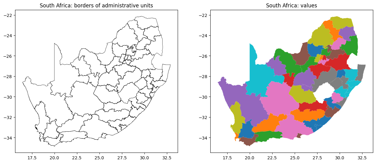
We could plot just the boundaries, or values attributed to each area.
fig, ax = plt.subplots(1, 2, figsize=(15,10))

# extract the boundary geometries
boundary_gdf = gdf_sa.boundary

# plot the boundary geometries
boundary_gdf.plot(ax=ax[0], color='black', lw=0.5)
ax[0].set_title('South Africa: borders of administrative units')

gdf_sa.plot(column='name', ax=ax[1])
ax[1].set_title('South Africa: values')

plt.show()
Saving Data#
You can save GeoDataFrames to various spatial data formats using the to_file() method:
gdf.to_file('path/to/output.shp')
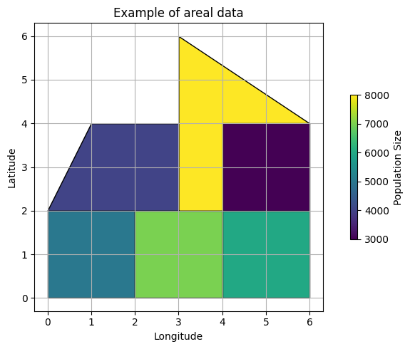
Create data manually#
If required, we can also create a geopandas data frame manually:
# create a GeoDataFrame with administrative boundaries (made-up data for illustration)
data = {'geometry': [Polygon([(0, 0), (0, 2), (2, 2), (2, 0)]),  # Polygon 1
                     Polygon([(2, 0), (2, 2), (4, 2), (4, 0)]),  # Polygon 2
                     Polygon([(0, 2), (1, 4), (3, 4), (3, 2)]),  # Polygon 3
                     Polygon([(3, 2), (3, 6), (6, 4), (5, 2)]),  # Polygon 4
                     Polygon([(4, 0), (4, 2), (6, 2), (6, 0)]),  # Polygon 5
                     Polygon([(4, 2), (4, 4), (6, 4), (6, 2)])],  # Polygon 6
        'Name': ['Admin District 1', 'Admin District 2', 'Admin District 3',
                 'Admin District 4', 'Admin District 5', 'Admin District 6'],  # Names of admin districts
        'Population': [5000, 7000, 4000, 8000, 6000, 3000]}  # Population counts for each admin district


gdf_toy = gpd.GeoDataFrame(data)
# plot the administrative boundaries with population size represented by color
fig, ax = plt.subplots(figsize=(8, 5))

# define colormap
cmap = plt.cm.viridis  # change the colormap here
norm = Normalize(vmin=gdf_toy['Population'].min(), vmax=gdf_toy['Population'].max())
sm = ScalarMappable(norm=norm, cmap=cmap)
sm.set_array([])  # necessary to use sm with plt.colorbar

# plot each administrative boundary with color based on population size
for idx, row in gdf_toy.iterrows():
    color = sm.to_rgba(row['Population'])
    gdf_toy.iloc[[idx]].plot(ax=ax, color=color, edgecolor='black')

# add colorbar with a shorter length
cbar = plt.colorbar(sm, ax=ax, shrink=0.5)  # adjust the shrink parameter to change the length of the color bar
cbar.set_label('Population Size')

plt.xlabel('Longitude')
plt.ylabel('Latitude')
plt.title('Example of areal data')
plt.grid(True)
plt.tight_layout()
plt.show()
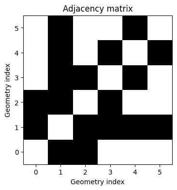
Adjancency structure#
Most models of areal data rely on the concept of adjacency matrix, i.e. a matrix \(A = (a_{ij})\) with entries
The adjacency matrix must be symmetric:
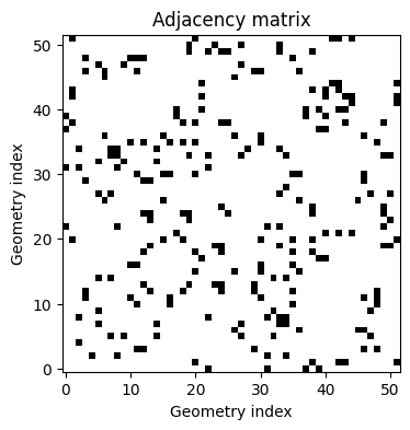
Let us compute adjacency matrix for the toy data, as well as the South Africa example.
def compute_adjacency_matrix(gdf):
    num_geometries = len(gdf)
    adjacency_matrix = np.zeros((num_geometries, num_geometries), dtype=int)

    for idx1, geometry1 in enumerate(gdf.geometry):
        for idx2, geometry2 in enumerate(gdf.geometry):
            if idx1 != idx2:
                if geometry1.touches(geometry2):  # check if geometries share a common boundary
                    adjacency_matrix[idx1, idx2] = 1

    return adjacency_matrix

def visualize_adjacency_matrix(matrix):
    plt.figure(figsize=(6, 4))
    plt.imshow(matrix, cmap='binary', origin='lower')
    plt.title('Adjacency matrix')
    plt.xlabel('Geometry index')
    plt.ylabel('Geometry index')
    plt.grid(False)
    plt.show()
adjacency_matrix_toy = compute_adjacency_matrix(gdf_toy)
adjacency_matrix_sa = compute_adjacency_matrix(gdf_sa)

# visualize the adjacency matrices
visualize_adjacency_matrix(adjacency_matrix_toy)
visualize_adjacency_matrix(adjacency_matrix_sa)
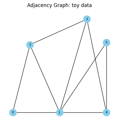
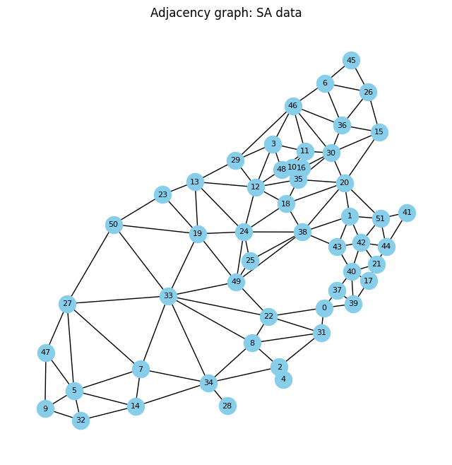
To understand adjacency, we can think about areal data as graphs with binary edges. Here each area represents a vertex in a graph, and an edge exists between vertices \(i\) and \(j\) if areas \(B_i\) and \(B_j\) share a border.
def adj_graph(gdf, size=(5,5), ttl='Adjacency Graph: toy data', plot=True):

    # create a empty graph
    nx_graph = nx.Graph()

    # add nodes with their coordinates and area names
    for idx, geometry in enumerate(gdf.geometry):
        centroid = geometry.centroid
        nx_graph.add_node(idx, pos=(centroid.x, centroid.y))

    adjacency_matrix = compute_adjacency_matrix(gdf)

    # add edges based on adjacency
    for i, j in zip(*np.where(adjacency_matrix == 1)):
        nx_graph.add_edge(i, j)

    # visualize the graph with nodes aligned with actual locations and labeled with area names
        pos = nx.get_node_attributes(nx_graph, 'pos')

    if plot:
        fig, ax = plt.subplots(1, 1, figsize=size)
        nx.draw(nx_graph, pos, with_labels=True, node_size=300, node_color="skyblue", font_size=8, font_color="black", ax=ax)
        plt.title(ttl)
        plt.show()

    return nx_graph, pos
_,_ = adj_graph(gdf_toy)
_,_ =adj_graph(gdf_sa, size=(8,8), ttl='Adjacency graph: SA data')
Models of areal data#
In models for areal data, the geographic units are denoted by \(B_i\), and the data are typically sums or averages of variables over these blocks. To introduce spatial association, we define a neighborhood structure based on the arrangement of the blocks in the map. Once the neighborhood structure is defined, one can construct models resembling autoregressive time series models, such as the intrinsic conditionally autoregressive model (ICAR, also called Besag) and conditionally autoregressive model (CAR).
All of the classical have the same functional form
and differ in how they define the precision matrix \(Q\).
The Besag, or ICAR, model#
The Besag, or ICAR (Intrinsic Conditional Autoregressive) model assumes that each location’s value is conditionally dependent on the values of its neighbors. This conditional dependency is often modeled as a weighted sum of the neighboring values, where the weights are determined by the neighborhood structure. Conditional mean of the random effect \(f_i\) is an average of its neighbours \(\{f_j \}_{j\sim i}\) and its precision is proportional to the number of neighbours. It describes the vector of spatially varying random effects \(f = (f_1, ..., f_n)^T\) using the prior \(f \sim \mathcal{N}(0, Q^-).\)
Here \(Q^-\) denotes the generalised inverse of matrix \(Q\), which, in turn, is computed as
\(D\) is a diagnoal matrix. It’s \(i\)-th element equals the total number of neighbours of area \(B_i\). Hence, \(D\) can be computed from \(A\):
Note that the structure matrix here can be viewed as graph Laplacian.
\(R\) is a rank-defficient matrix. It is recommended, for example, to place an adidtional constraint, such sum-to-zero constraint on each non-singleton connected component:
Conditional Autoregressive Models (CAR)#
Similar to ICAR, the CAR model assumes that the value of a variable in one area depends on the values of neighboring areas, with weights specified by a spatial adjacency matrix. However, it introcues an additional parameter \(\alpha\), allowing to estimate the amount of spatial correlation.
The spatial random effect now is modelled as
with
If \(\alpha=0\), the model consist only of i.i.d. random effects, and if \(\alpha\) is close to 1, the model approaches ICAR.
Here is an artificial example of the CAR model:
def expit(x):
    return 1/(1 + jnp.exp(-x))

def car_model(y, A):

    n = A.shape[0]
    d = jnp.sum(A, axis=1)
    D = jnp.diag(d)

    b0 = numpyro.sample('b0', dist.Normal(0,1).expand([n]))
    tau = numpyro.sample('tau', dist.Gamma(3, 2))
    alpha = numpyro.sample('alpha', dist.Uniform(low=0., high=0.99))

    Q_std = D - alpha*A
    car_std = numpyro.sample('car_std', dist.MultivariateNormal(loc=jnp.zeros(n), precision_matrix=Q_std))
    sigma = numpyro.deterministic('sigma', 1./jnp.sqrt(tau))
    car = numpyro.deterministic('car', sigma * car_std)

    lin_pred = b0 + car
    p = numpyro.deterministic('p', expit(lin_pred))

    # likelihood
    numpyro.sample("obs", dist.Bernoulli(p), obs=y)


# spatial data 'y' and adjacency structure 'adj'
y = jnp.array([0, 0, 1, 0, 1, 0, 0, 0])

A = np.array([[0, 1, 0, 0, 0, 0, 0, 0],
              [1, 0, 1, 1, 0, 0, 0, 1],
              [0, 1, 0, 1, 0, 0, 0, 1],
              [0, 1, 1, 0, 1, 0, 0, 1],
              [0, 0, 0, 1, 0, 0, 0, 0],
              [0, 0, 0, 0, 0, 0, 1, 0],
              [0, 0, 0, 0, 0, 1, 0, 1],
              [0, 1, 1, 1, 0, 0, 1, 0]])

# Run MCMC to infer the parameters
nuts_kernel = NUTS(car_model)
mcmc = MCMC(nuts_kernel, num_samples=1000, num_warmup=1000, progress_bar=False)
mcmc.run(rng_key=jax.random.PRNGKey(0), y=y, A=A)

# Extract posterior samples
samples = mcmc.get_samples()

#mcmc.print_summary()
Task 28
Simulate data from the CAR model using South African boundaries and neighbourhood structure (use
adjacency_matrix_saasA, andy=Noneto create simulations) with Bernoulli likelihoodFit the CAR model to the data which you have simluated (make adjustments if necessary).
Plot posterior distribution of \(\alpha\), and add the true velue of \(\alpha\) to this plot. What do you observe?
Make sactter plots of \(f_\text{true}\) vs \(f_\text{fitted}\), and add a diagonal line to this plot. What do you observe?
The Besag-Yorg-Mollié model#
The Besag, York, and Mollié (BYM) decomposes the spatial random effect \(f\) into the sum of an i.i.d. component \(v\) and spatiallly structured component \(w\). Each of these two components has its own precision parameter \(\tau_v\) and \(\tau_w\), respectively:
where the \(R\) is responsible for the ICAR components, i.e. \(R = D - A\).
This model provides more flexibility than the CAR formulation.